5.7 KiB

Raw Blame History Unescape Escape

3.2.9 时间序列的高级应用

代码	描述
D	天（calendar day，按日历算，含双休日）
W	周（weekly） M 月末（month end）
Q	季末（quarter end）
A	年末（year end）
H	小时（hours）
T	分钟（minutes）
S	秒（seconds）
L	毫秒（milliseonds）
U	微秒（microseconds）
N	纳秒（nanoseconds）
B	天（business day，仅含工作日）
BM	月末（business month end，仅含工作日）
BQ	季末（business quarter end，仅含工作日）
BA	年末（business year end，仅含工作日）
BH	小时（business hours，工作时间）
MS	月初（month start）
BMS	月初（business month start，仅含工作日）
QS	季初（quarter start）
BQS	季初（business quarter start，仅含工作日）
AS	年初（year start）
BAS	年初（business year start，仅含工作日）

时间频率与偏移量

我们可以在频率代码后面加三位月份缩写字母来改变季、年频率的开始时间，也可以再后面加三位星期缩写字母来改变一周的开始时间：

Q-JAN、BQ-FEB、QS-MAR、BQS-APR 等
W-SUN、W-MON、W-TUE、W-WED 等

时间频率组合使用：

In[0]：pd.timedelta_range(0,periods=9,freq="2H30T")
Out[0]：TimedeltaIndex(['00:00:00', '02:30:00', '05:00:00', '07:30:00', '10:00:00', '12:30:00', '15:00:00', '17:30:00', '20:00:00'], dtype='timedelta64[ns]', freq='150T')

比如直接创建一个工作日偏移序列：

In[1]：from pandas.tseries.offsets import BDay 
 	  pd.date_range('2015-07-01', periods=5, freq=BDay())
Out[1]：DatetimeIndex(['2015-07-01', '2015-07-02', '2015-07-03', '2015-07-06', '2015-07-07'], dtype='datetime64[ns]', freq='B')

重新取样、迁移和窗口

重新取样

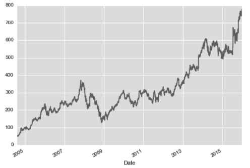
处理时间序列数据时，经常需要按照新的频率（更高频率、更低频率）对数据进行重新取样。举个例子，首先通过pandas—datareader程序包(需要手动安装)导入 Google 的历史股票价格，只获取它的收盘价：

In[2]： 
from pandas_datareader import data
goog = data.DataReader('GOOG',start="2014",end="2016",data_source="google")['Close']   # Close表示收盘价的列
In[3]： 
import matplotlib.pyplot as plt 
import seaborn; seaborn.set()
goog.plot();   #数据可视化

输出：

我们可以通过resample()方法和asfreq()方法解决这个问题，resample() 方法是以数据累计为基础，而asfreq()方法是以数据选择为基础。

In[4]： 
goog.plot(alpha=0.5, style='-') 
goog.resample('BA').mean().plot(style=':') 
goog.asfreq('BA').plot(style='--'); 
plt.legend(['input', 'resample', 'asfreq'], loc='upper left');

输出：

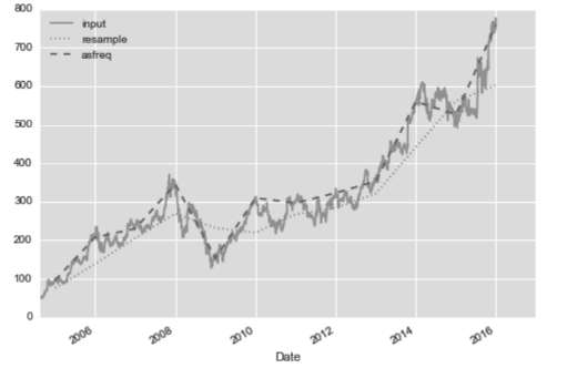
请注意这两种取样方法的差异：在每个数据点上，resample反映的是上一年的均值，而asfreq反映的是上一年最后一个工作日的收盘价。

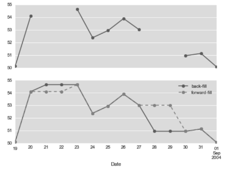
数据集中经常会出现缺失值，从上面的例子来看，由于周末和节假日股市休市，周末和节假日就会产生缺失值，上面介绍的两种方法默认使用的是向前取样作为缺失值处理。与前面介绍过的pd.fillna()函数类似，asfreq()有一个method参数可以设置填充缺失值的方式。

In[5]：fig, ax = plt.subplots(2, sharex=True) 
	   data = goog.iloc[:10] 
	   data.asfreq('D').plot(ax=ax[0], marker='o') 
	   data.asfreq('D', method='bfill').plot(ax=ax[1], style='-o') 
	   data.asfreq('D', method='ffill').plot(ax=ax[1], style='--o') 
	   ax[1].legend(["back-fill", "forward-fill"]);

输出：

时间迁移

另一种常用的时间序列操作是对数据按时间进行迁移，Pandas有两种解决这类问题的方法：shift()和tshift()。简单来说，shift()就是迁移数据，而 tshift()就是迁移索引。两种方法都是按照频率代码进行迁移。

下面我们将用shift() 和tshift()这两种方法让数据迁移900天：

In[6]：fig, ax = plt.subplots(3, sharey=True) 
	   # 对数据应用时间频率，用向后填充解决缺失值
	   goog = goog.asfreq('D', method='pad') 
	   goog.plot(ax=ax[0]) 
	   goog.shift(900).plot(ax=ax[1]) 
	   goog.tshift(900).plot(ax=ax[2]) 
	   # 设置图例与标签
	   local_max = pd.to_datetime('2007-11-05') 
	   offset = pd.Timedelta(900, 'D') 
	   ax[0].legend(['input'], loc=2) 
	   ax[0].get_xticklabels()[4].set(weight='heavy', color='red') 
	   ax[0].axvline(local_max, alpha=0.3, color='red') 
	   ax[1].legend(['shift(900)'], loc=2) 
	   ax[1].get_xticklabels()[4].set(weight='heavy', color='red') 
	   ax[1].axvline(local_max + offset, alpha=0.3, color='red') 
	   ax[2].legend(['tshift(900)'], loc=2)
	   ax[2].get_xticklabels()[1].set(weight='heavy', color='red') 
 	   ax[2].axvline(local_max + offset, alpha=0.3, color='red');

输出：

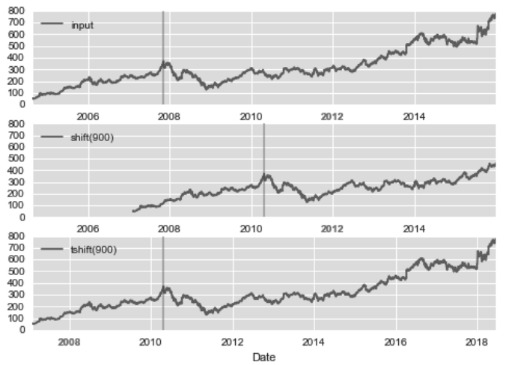
shift(900)将数据向前推进了900天，这样图形中的一段就消失了（最左侧就变成了缺失值），而tshift(900)方法是将时间索引值向前推进了900天。

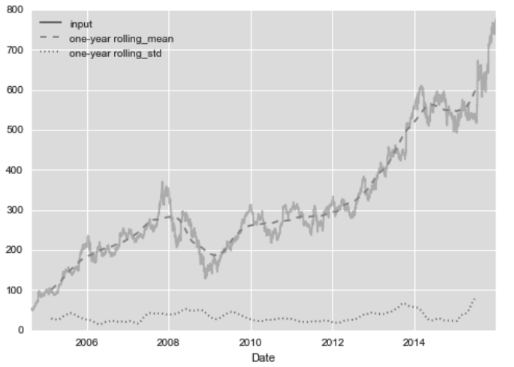
移动时间窗口

Pandas处理时间序列数据的第3种操作是移动统计值。这些指标可以通过 Series和DataFrame的rolling()属性来实现，它会返回与groupby操作类似的结果，移动视图使得许多累计操作成为可能。

In[7]： rolling = goog.rolling(365, center=True) 
 		data = pd.DataFrame({'input': goog, 'one-year rolling_mean': rolling.mean(), 'one-year rolling_std': rolling.std()}) 
 		ax = data.plot(style=['-', '--', ':']) 
 		ax.lines[0].set_alpha(0.3)

输出：

5.7 KiB Raw Blame History Unescape Escape