pt5jvslni/Chapter12/使用sklearn实现欺诈检测功能.md

12.4 使用sklearn实现欺诈检测功能

前两节已经解决掉了这个数据集的两个难点，那么接下来，要做的事情就是一些非常基本的处理，来对该数据集进行建模，从而实现欺诈检测的功能了。

不过在建模之前，我们需要对 Time 和 Amount 这两个特征进行分析和处理。

首选是 Time ，可以看看 Time 的一个分布。

transactions['Time'].describe()

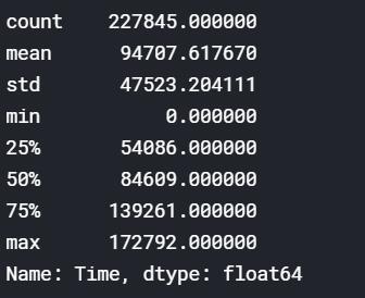
Time 特征的值是比较大的数，看起来像是以秒为单位的时间戳。那么这个时候我们可以将该时间戳转换成分钟和小时。

# 将Time转换成秒为单位的时间戳
timedelta = pd.to_timedelta(transactions['Time'], unit='s')
# 创建一个新的特征Time_min，表示分钟
transactions['Time_min'] = (timedelta.dt.components.minutes).astype(int)
# 创建一个新的特征Time_hour，表示小时
transactions['Time_hour'] = (timedelta.dt.components.hours).astype(int)

然后是 Amount 特征，同样，先看看分布。

transactions['Amount'].describe()

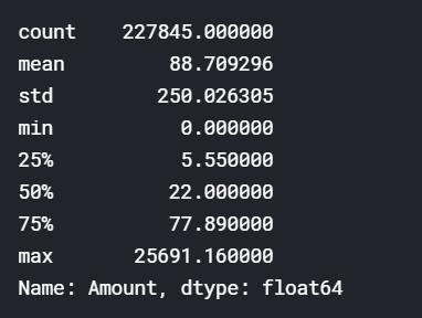
从分布来看，Amount 特征好像存在着严重的倾斜。我们把直方图画出来验证一下我们的猜测。

plt.figure(figsize=(12,4), dpi=80)
sns.distplot(transactions['Amount'], bins=300, kde=False)
plt.ylabel('Count')
plt.title('Transaction Amounts')

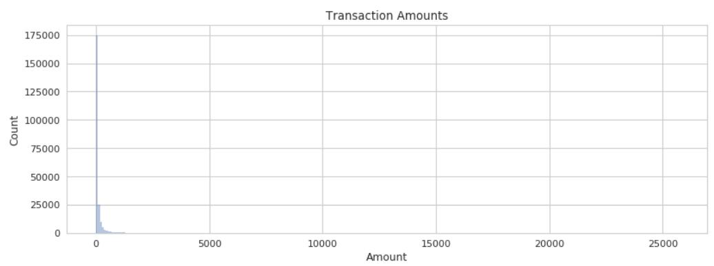
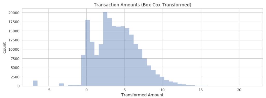
果然！大量数据的 Amount 都接近于 100 左右。一般在碰到这种倾斜严重的特征时，我们需要对它进行 log 变换，log 变换的意图就是将倾斜严重的分布，尽量让它变得更均匀。

transactions['Amount_log'] = np.log(transactions.Amount + 0.01)

然后再可视化一下，可以看出经过 log 变换之后，分布变得更加均匀了。

接下来可以使用我们的特征来构造欺诈检测模型了。构建模型很简单，使用 sklearn 提供的接口即可。

# 导入imblearn中的pipeline功能
from imblearn.pipeline import make_pipeline as make_pipeline_imb 
# 导入上一节中提到的SMOTE功能
from imblearn.over_sampling import SMOTE

# 选用一些特征
transactions = transactions[["Time_hour","Time_min","V2","V3","V4","V9","V10","V11","V12","V14","V16","V17","V18","V19","V27","Amount_log","Class"]]

# 构建pipeline，pipeline的意思是流水线，在这个欺诈检测的流水线中做了两件事情
# 1. SMOTE过采样
# 2. 使用决策树来进行分类，即欺诈检测
smote_pipeline = make_pipeline_imb(SMOTE(), DecisionTreeClassifier()
)

有了 pipeline 之后，我们就相当于已经有了一条能够检测欺诈交易的流水线了。不过这样一条流水线的效果好不好，需要使用数据来进行验证。下一节中将会向你介绍怎样验证算法的效果。